Histograms#
matviz provides two main histogram functions:
nhist— smart 1D histograms with automatic binningndhist— 2D density histograms (heat maps)
Both use Scott’s normal reference rule for bin selection and handle edge cases gracefully.
import numpy as np
import matplotlib.pyplot as plt
from matviz.histogram_utils import nhist, ndhist
from matviz.viz import subplotter, title
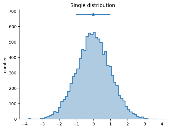
nhist — 1D Histograms#
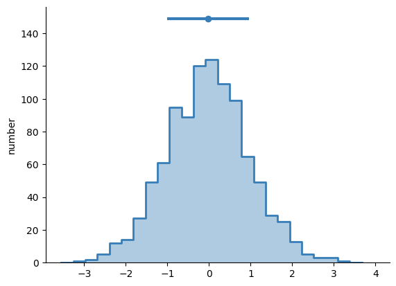
Single array#
y = np.random.randn(10000)
fig = nhist(y)
title('Single distribution')
plt.show()
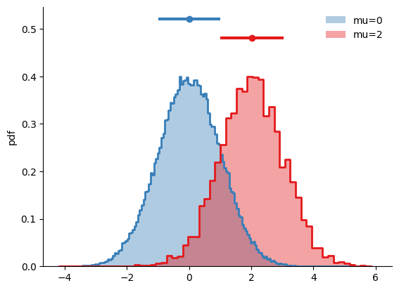
Dictionary input — compare distributions#
A = {'mu=0': np.random.randn(100000), 'mu=2': np.random.randn(5000) + 2}
fig = nhist(A)
plt.show()
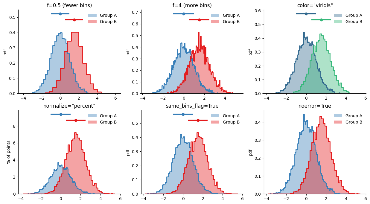
Key parameters#
A = {'Group A': np.random.randn(10000), 'Group B': np.random.randn(5000) + 1.5}

plt.figure(figsize=(15, 8))

subplotter(2, 3, 0)
nhist(A, f=0.5)
title('f=0.5 (fewer bins)')

subplotter(2, 3, 1)
nhist(A, f=4)
title('f=4 (more bins)')

subplotter(2, 3, 2)
nhist(A, color='viridis')
title('color="viridis"')

subplotter(2, 3, 3)
nhist(A, normalize='percent')
title('normalize="percent"')

subplotter(2, 3, 4)
nhist(A, same_bins_flag=True)
title('same_bins_flag=True')

subplotter(2, 3, 5)
nhist(A, noerror=True)
title('noerror=True')

plt.show()
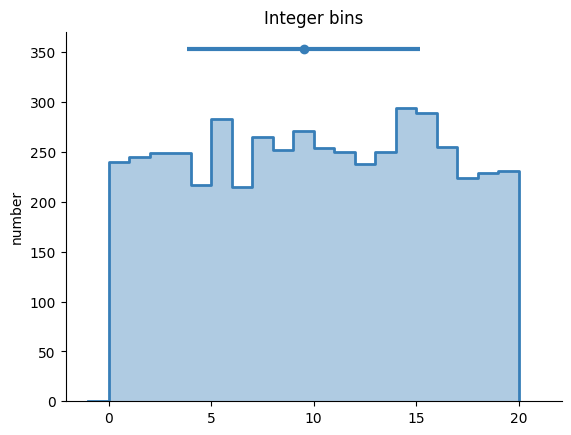
Integer bins and axis limits#
integers = np.random.randint(0, 20, 5000)
fig = nhist(integers, int_bins_flag=True)
title('Integer bins')
plt.show()
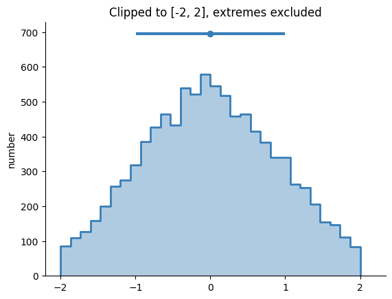
data = np.random.randn(10000)
fig = nhist(data, minx=-2, maxx=2, exclude_extremes=True)
title('Clipped to [-2, 2], extremes excluded')
plt.show()
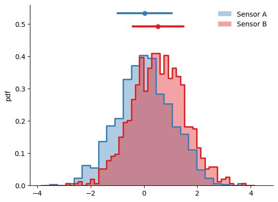
DataFrame input#
import pandas as pd

df = pd.DataFrame({
    'Sensor A': np.random.randn(1000),
    'Sensor B': np.random.randn(1000) + 0.5,
})
fig = nhist(df)
plt.show()
Accessing return data#
fig = nhist(np.random.randn(1000))
print('Bin counts:', fig.nhist['N'][0][:5], '...')
print('Bin edges:', fig.nhist['bins'][0][:5], '...')
plt.show()
Bin counts: [ 0  1  2  5 12] ...
Bin edges: [-3.55368336 -3.26462916 -2.97557496 -2.68652076 -2.39746656] ...
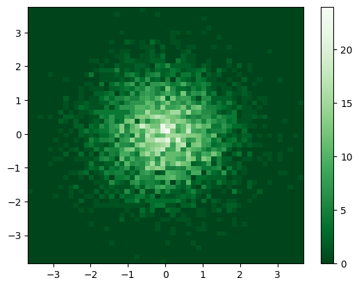
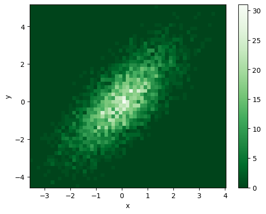
ndhist — 2D Histograms#
Basic 2D histogram#
x = np.random.randn(5000)
y = x + np.random.randn(5000)
fig = ndhist(x, y)
plt.colorbar()
plt.xlabel('x')
plt.ylabel('y')
plt.show()
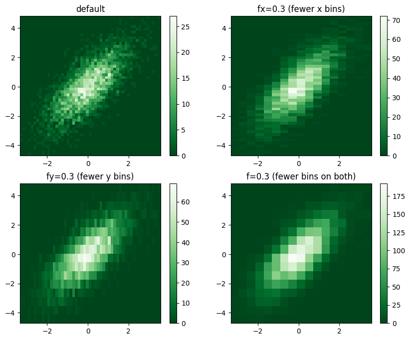
Bin density with f, fx, fy#
The f parameter controls bin density relative to the default (Scott’s rule).
Use fx and fy to control x and y axes independently.
x = np.random.randn(5000)
y = x + np.random.randn(5000)

plt.figure(figsize=(10, 8))

subplotter(2, 2, 0)
ndhist(x, y)
title('default')
plt.colorbar()

subplotter(2, 2, 1)
ndhist(x, y, fx=0.5)
title('fx=0.3 (fewer x bins)')
plt.colorbar()

subplotter(2, 2, 2)
ndhist(x, y, fy=0.5)
title('fy=0.3 (fewer y bins)')
plt.colorbar()

subplotter(2, 2, 3)
ndhist(x, y, f=0.5)
title('f=0.3 (fewer bins on both)')
plt.colorbar()

plt.show()
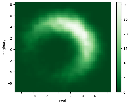
Complex numbers#
z = (5 + np.random.randn(10000)) * np.exp(1j * (np.random.randn(10000) + np.pi/4))
fig = ndhist(z, smooth=1)
plt.colorbar()
plt.xlabel('Real')
plt.ylabel('Imaginary')
plt.show()
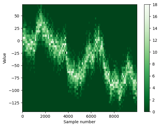
Time series mode#
n = 10000
y = np.cumsum(np.random.randn(n)) + 15 * np.random.randn(n)
fig = ndhist(y, fx=5)
plt.xlabel('Sample number')
plt.ylabel('Value')
plt.colorbar()
plt.show()
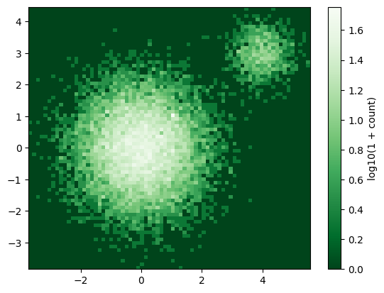
Log colorbar#
x = np.concatenate([np.ones(50), np.random.randn(15000), 4 + np.random.randn(1000)/2])
y = np.concatenate([np.ones(50), np.random.randn(15000), 3 + np.random.randn(1000)/2])
fig = ndhist(x, y, log_colorbar_flag=True)
plt.colorbar(label='log10(1 + count)')
plt.show()
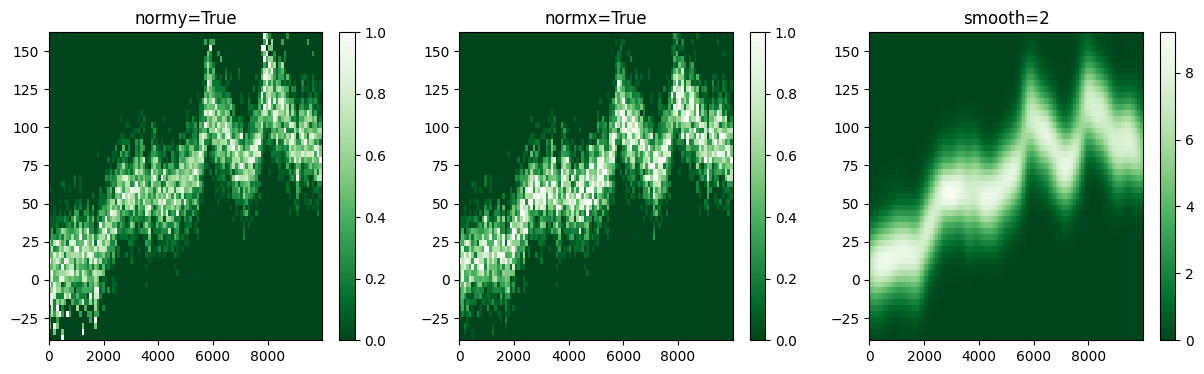
Normalization and smoothing#
n = 10000
y = np.cumsum(np.random.randn(n)) + 15 * np.random.randn(n)

plt.figure(figsize=(15, 4))

subplotter(1, 3, 0)
ndhist(y, fx=5, normy=True)
title('normy=True')
plt.colorbar()

subplotter(1, 3, 1)
ndhist(y, fx=5, normx=True)
title('normx=True')
plt.colorbar()

subplotter(1, 3, 2)
ndhist(y, fx=5, smooth=2)
title('smooth=2')
plt.colorbar()

plt.show()
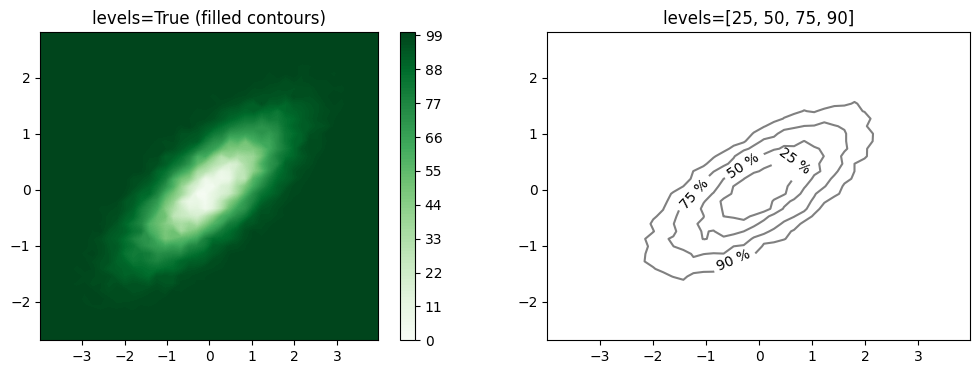
Contour levels#
x = np.random.randn(50000)
y = x * 0.5 + np.random.randn(50000) * 0.5

plt.figure(figsize=(12, 4))

subplotter(1, 2, 0)
ndhist(x, y, f=0.5, levels=True)
title('levels=True (filled contours)')
plt.colorbar()

subplotter(1, 2, 1)
ndhist(x, y, f=0.5, levels=[25, 50, 75, 90])
title('levels=[25, 50, 75, 90]')

plt.show()
Accessing return data#
fig = ndhist(np.random.randn(5000), np.random.randn(5000))
print('Counts shape:', fig.ndhist['counts'].shape)
print('bins_x length:', len(fig.ndhist['bins_x']))
print('bins_y length:', len(fig.ndhist['bins_y']))
plt.colorbar()
plt.show()
Counts shape: (56, 57)
bins_x length: 57
bins_y length: 58